
Direct costs are itemized for all necessary parts of the project. Direct costs are all of the costs which can be attributed directly to the project. Direct costs include costs for general requirements (Division 1 of MasterFormat), which includes such items as project management and coordination, quality control, temporary facilities and controls, cleaning and waste management.[35] Direct costs may also include the costs of project planning, investigation, studies, and design; land or right of way acquisition, and other non-construction costs. Usually, a subtotal of total direct costs is provided in the estimate.
An order-of-magnitude estimate is prepared when little or no design information is available for the project. It is called order of magnitude because that may be all that can be determined at an early stage. In other words, perhaps we can only determine that it is of a 10,000,000 magnitude as opposed to a 1,000,000 magnitude. Various techniques are employed for these estimates, including experience and judgment, historical values and charts, rules of thumb, and simple mathematical calculations.[36] Factor estimating is one of the more popular methods. This involves taking the known cost of a similar facility and factoring the cost for size,[37] place, and time. Cost modeling is another common technique. In cost modeling the estimator models the various parameters of the facility and applies costs to the derived scope.
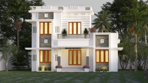
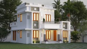
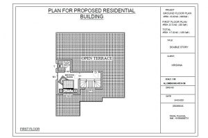
Total Area : 1259 Square Feet
Client : Krishna Das
Designer : Faisal Pulikkal
Mob & What Sapp : +91 99468 65731
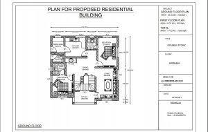
Ground Floor : 1003 Square Feet
Sit out
Living room
Dining area
2 Bedroom with attached bathroom
Kitchen
Work area
1 Common bathroom
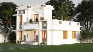
First Floor : 255 Square Feet
Upper passage
1 Bedroom with attached bathroom
Open balcony
Open terrace
With only one variable input in the short run, each possible quantity of output requires a specific quantity of usage of labor, and the short–run total cost as a function of the output level is this unique quantity of labor times the unit cost of labor. But in the long run, with the quantities of both labor and physical capital able to be chosen, the total cost of producing a particular output level is the result of an optimization problem: The sum of expenditures on labor (the wage rate times the chosen level of labor usage) and expenditures on capital (the unit cost of capital times the chosen level of physical capital usage) is minimized with respect to labor usage and capital usage, subject to the production function equality relating output to both input usages; then the (minimal) level of total cost is the total cost of producing the given quantity of output.
The average total cost curve is constructed to capture the relation between cost per unit of output and the level of output, ceteris paribus. A perfectly competitive and productively efficient firm organizes its factors of production in such a way that the usage of the factors of production is as low as possible consistent with the given level of output to be produced. In the short run, when at least one factor of production is fixed, this occurs at the output level where it has enjoyed all possible average cost gains from increasing production. This is at the minimum point in the above diagram.
The long-run marginal cost curve is shaped by returns to scale, a long-run concept, rather than the law of diminishing marginal returns, which is a short-run concept. The long-run marginal cost curve tends to be flatter than its short-run counterpart due to increased input flexibility. The long-run marginal cost curve intersects the long-run average cost curve at the minimum point of the latter.:208 When long-run marginal cost is below long-run average cost, long-run average cost is falling (as additional units of output are considered).